While Excel is easily one of Microsoft’s most useful products, many people don’t know how to get the most out of it, and we often get asked how to make a Pivot Table. Whether you’re tracking sales, organizing expenses, managing inventory, or analyzing customer information, Pivot Tables can help turn large amounts of information into something much easier to understand. I will admit that I love spreadsheets, and they are by far one of the most powerful tools available, used by businesses of all sizes every day.
What is a Pivot Table?
A Pivot Table is a feature in Excel that allows you to create a manipulable matrix to view, organize, summarize, and analyze large sets of data. Instead of sorting through hundreds or thousands of rows manually, a Pivot Table can quickly calculate totals, averages, counts, and other useful statistics, making it much easier to identify trends and patterns that may not be obvious when looking at raw data alone. It is invaluable for those of us who like to stay organized through Excel, and businesses frequently use Pivot Tables to compare sales performance, track spending, analyze productivity, and create management reports.
In this blog, I’m going to explain how to use Pivot Tables in simple terms to get the most out of them.
Collect Your Data
Before we can do anything, we’ll need a data set with multiple rows and columns in order to make a Pivot Table. Important note: the more organized your information is before you get started, the easier it will be to build and analyze your results. It is absolutely worth spending a few extra minutes cleaning up your data, as it will save you a great deal of frustration later.
So let’s talk about cleaning it up, because how you organize the data is essential. For the sake of ease, always use the first row to label the data in each column; clear labels make it easier for Excel to recognize and organize your information when creating a Pivot Table. Every column should contain a single type of information, such as dates, employee names, product names, or dollar amounts.
Anyone who uses Excel regularly will tell you that it works best when the information is clearly labeled and consistently formatted, like this:
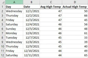
Notice that I keep the dates in columns rather than rows because Excel tends to assume this is the way you will format your data, and it is a much more user-friendly style. It also makes it easier to automatically identify relationships between different pieces of information when building reports and summaries.
Insert Pivot Table
Once your dataset is complete and organized to your preference, click and highlight all the cells to be included in your Pivot Table. With the cells highlighted, go into the Insert tab on the top banner and then click the icon labeled PivotTable. A pop-up screen will appear that offers several options for the table. The first section of the pop-up wizard provides the option to change or add data to the set, but if you highlighted the information before clicking the icon, this should be auto-populated and require little or no adjustment.
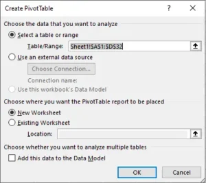 The next section lets you decide where you want the Pivot Table located, which defaults to creating a new worksheet, which is essentially just a second tab that you can find at the bottom-left of the page. It typically gets automatically titled Sheet2, but you can rename it to whatever you want. Creating the Pivot Table on a separate worksheet is the easiest option, especially if you are new to it, because it gives you more room to work and keeps your original data untouched. If you prefer the Pivot Table to be located somewhere else, you can click the box labeled “Location” and then click the cell where you want the top-left corner of your table to be located. Changing the location can be useful if you are building a dashboard or report where you want multiple Pivot Tables and charts displayed on the same worksheet.
Newer versions of Excel provide some options for Recommended Pivot Tables, which analyze your data and suggest several useful layouts automatically. These recommended PivotTables can be a great starting point for beginners because the program does much of the initial setup for you.
Pivot Table Fields
Once you hit OK on the Create Pivot Table wizard, all the fields that can be used to create the table are displayed on the right side of the page. These fields represent the column headings from your original dataset, and by moving them into different sections, you control how Excel summarizes and displays the information. The first step is to select what you want to analyze from the data.
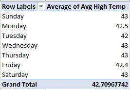 In my example, I want to know the average temperature on a Monday in December, so I click on the Day option and drag it into the Rows box, and then any field placed in the Rows area becomes a category that helps organize the information. After that, I want the value for each day to be the average high temperature, so I drag that option into the Values box. The Values area is where Excel performs calculations such as sums, averages, counts, minimums, and maximums.
Sometimes things don’t do what you think, for example, it may default to a sum of the temperatures. If that happens, you can fix it by clicking the dropdown on the item in the Values box, clicking Value Field Settings, and changing the formula type. To change the format of the setting, click on the Number Format button in this pop-up; it allows you to display currency, percentages, dates, or other formats that better fit your data.
When we are done, the Pivot Table tells us that the average Wednesday in December in Hagerstown, MD is 43 degrees.
Using Filters and Columns
One of the most useful features of a Pivot Table is the ability to view the same data from multiple perspectives without changing the original spreadsheet. We do this by dragging fields into the Columns and Filters sections to reorganize the information quickly. It is this flexibility that gives Pivot Tables their name.
For example, you could put Month in the Columns section and Year in the Filters section, which would allow you to compare monthly trends while still being able to narrow your results to a specific year. That’s one of the great things about Pivot Tables: with only a few clicks, you can answer questions that would otherwise require multiple formulas and manual calculations.
Using Microsoft Copilot to Create Pivot Tables
Microsoft has also begun integrating Copilot AI into Excel, making Pivot Tables even easier to create. Instead of manually selecting fields and building reports, Copilot can analyze your data and generate Pivot Tables based on natural language requests. For those who are unfamiliar with the interface or are looking for ways to generate reports more quickly, using AI can be particularly useful.
For example, you can ask Copilot to “Create a Pivot Table showing total sales by product category” or “Show average monthly expenses by department,” and Copilot will analyze the available data and generate a Pivot Table based on your request. If the results are not exactly what you need, you can continue refining your request until the report displays the information you want.
While Copilot can save time and simplify the process, I still recommend learning the fundamentals of Pivot Tables. Understanding how Rows, Columns, Values, and Filters work will help you verify the results and make adjustments when necessary. AI is a helpful tool, but it works best when paired with a solid understanding of the underlying feature.
What Else Can I Do in Excel?
Pivot Tables are just one example of the many organizational and analytical features that Excel offers. As you have seen, they can be used to summarize sales reports, analyze budgets, monitor inventory, track customer activity, and much more. I can tell you from experience, once you become comfortable with them, you’ll find yourself using them whenever you need to make sense of large amounts of information.
Keep an eye out for more upcoming tutorials for Excel, and should you need any tips or advice sooner, never hesitate to give us a call at 301-456-6931 or send us an email at [email protected].
